Lock-in amplifier simulation in Python: settling, noise bandwidth and a Bode sweep
By Alex Hernandez · · 14 min read
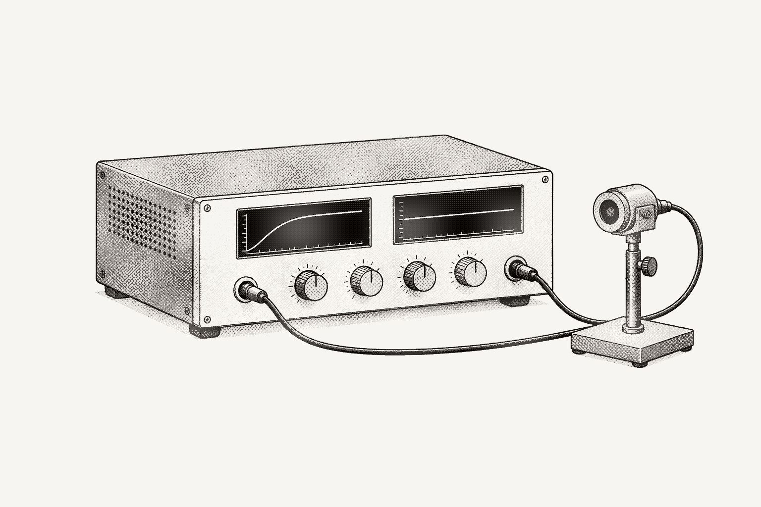
To simulate a lock-in amplifier, wire a simulated dual-phase lock-in to a bench that carries your signal and run the PyVISA script you will use on the real unit. The simulation settles as an order-n exponential in virtual time and filters noise by its equivalent noise bandwidth, so waits, ranges and error handling are proven first.
EdgeSim is the open-source bench simulator from Galois Labs: simulated instruments wired into simulated benches that PyVISA scripts, pytest, galois-edge and AI agents can't tell from real hardware. This guide drives its lock-in, galois_sim-lockin-1, on the shipped bench lockin.bench.yaml, an RC low-pass that the lock-in's own SINE_OUT drives, plus two small benches shown in full. The EdgeSim announcement places the lock-in among the other classes. Every snippet and output ran against EdgeSim 0.2.0; EdgeSim's open-source release, with the edgesim package and its example benches, is coming soon. Behavior claims come from the profile, its plugin and their tests, which are public with the release; the detection principle follows (Source: Stanford Research Systems, Application Note #3, About Lock-In Amplifiers).
What does the simulated lock-in model?
A lock-in multiplies its input by a reference sine and by the same sine shifted 90 degrees, then low-pass filters both products. Stanford Research Systems puts it this way: "Lock-in amplifiers use a technique known as phase-sensitive detection to single out the component of the signal at a specific reference frequency and phase." The outputs are X = V·cos θ and Y = V·sin θ, the magnitude R and the phase θ.
The simulation reads the net on SIG_IN as spectral lines: sines, squares and ramps in closed form, and arb, prbs and clip numerically. It demodulates the lines against the reference and applies the filter exactly, so nothing is sampled per sample in Python. Readings are input-referred rms volts and θ is in degrees. Sensitivity sets the full scale of the overload flags and the auto-gain ladder, not the scaling of X, Y and R.
| Setting | Range and steps | SCPI |
|---|---|---|
| Reference | Internal, 1 mHz to 500 kHz, or external on REF_IN; harmonic n from 1 to 99 with n × f at most 500 kHz | :REFerence:SOURce, :FREQuency, :HARMonic, :PHASe |
| Sensitivity | 2 nV to 1 V, 1-2-5 ladder, 27 steps | :INPut:SENSitivity |
| Time constant | 10 µs to 30 ks, 1-3 ladder, 20 steps | :FILTer:TCONstant |
| Slope | 6, 12, 18 or 24 dB/oct, which is 1 to 4 poles | :FILTer:SLOPe |
| Coupling | DC, or AC with a 0.16 Hz high-pass | :INPut:COUPling |
| Outputs | X, Y, R, THETa; SNAP? reads up to four at one instant | :MEASure:R?, :MEASure:SNAP? R,THETa |
| Auto and flags | Auto phase, auto gain, overload bits 1 input and 2 output | :AUTO:PHASe, :AUTO:GAIN, :STATus:OVERload? |
A SCPI write to a ladder setting snaps to the nearest rung on a log scale: 0.3 V of sensitivity stores 0.2 V.
How do I open the lock-in bench from Python?
The shipped bench wires the lock-in's SINE_OUT to a 1 kΩ and 100 nF low-pass, returns the filter's output to SIG_IN, and puts a DMM on the same net. The reference is the internal oscillator at the same frequency, so the low-pass's phase appears directly as θ:
    ext:
      sim:
        profile: galois_sim-lockin-1
        state: {reference.frequency: 1591.55, sine_out.amplitude: 1.0, filter.time_constant: 0.03, filter.slope: "24"}
edges:
  - {id: e-drive, source: inst-lockin-sim1, target: fn-in, ..., ext: {sim: {sourcePort: SINE_OUT}}}
  - {id: e-sense, source: fn-out, target: inst-lockin-sim1, ..., ext: {sim: {targetPort: SIG_IN}}}
The corner is 1 / (2π · 1 kΩ · 100 nF) = 1591.55 Hz. At the corner a 1 Vrms drive gives R = 1 / √2 V and θ = −45°. The scripts share one helper:
import pyvisa


def open_lockin(bench="lockin.bench.yaml", port=5025):
    rm = pyvisa.ResourceManager(f"{bench}@edgesim")
    lia = rm.open_resource(f"TCPIP0::127.0.0.1::{port}::SOCKET", read_termination="\n", write_termination="\n")
    return rm, lia, lia.visalib.world


def snap(lia, *names):
    """SNAP? reads up to four of X, Y, R, THETa at the same instant."""
    return [float(v) for v in lia.query(":MEASure:SNAP? " + ",".join(names)).split(",")]


def drain(inst):
    """Every queued error, oldest first."""
    queue = []
    while not (e := inst.query(":SYSTem:ERRor?")).startswith("0,"):
        queue.append(e)
    return queue
world.advance(seconds) moves virtual time on the bench's stepped clock; it is the one simulator-only call, and a real script sleeps where these scripts advance.
How long does the output take to settle?
After any change the filter output follows the order-n exponential. For n poles of time constant T and x = t / T, the fraction of a step still unsettled is e−x · Σ xk / k! for k below n. settle.py switches SINE_OUT on at the corner, with a 30 ms time constant and 24 dB/oct, and reads R along the way:
import math

from lia import open_lockin

LIA = "sim-lockin-1"
rm, lia, world = open_lockin()
lia.write(":SOURce:VOLTage 0.5")                  # 0.5 Vrms drive, as in the sweep below
lia.write(":OUTPut:STATe OFF")                    # SINE_OUT off: the RC and the lock-in input sit at zero
world.advance(2.0)
tc, poles = float(lia.query(":FILTer:TCONstant?")), round(float(lia.query(":FILTer:SLOPe?")) / 6)
print(f"filter: {tc} s x {poles} poles ({lia.query(':FILTer:SLOPe?')} dB/oct), ENBW {float(lia.query(':FILTer:ENBW?')):.4f} Hz, "
      f"settling to 99 % {float(lia.query(':FILTer:SETTling?')):.4f} s")

lia.write(":OUTPut:STATe ON")                     # the step: the signal appears at t = 0
r_final = 0.5 * (5e6 / (5e6 + 1050)) / math.sqrt(2)   # 0.5 Vrms through the RC at its corner (-3 dB) and the 50 ohm + 5 Mohm divider
print(f"{'t / T':>7} {'t / s':>7} {'R read / mV':>12} {'R formula / mV':>15}")
elapsed = 0.0
for k in (0, 0.5, 1, 2, 4, 6, 10.045, 14, 20):
    world.advance(k * tc - elapsed)               # virtual time moves only here
    elapsed = k * tc
    remaining = math.exp(-k) * sum(k**j / math.factorial(j) for j in range(poles))
    print(f"{k:7.3f} {k * tc:7.4f} {float(lia.query(':MEASure:R?')) * 1e3:12.4f} {r_final * (1 - remaining) * 1e3:15.4f}")

console = world.state(LIA, "demod")["demod.r"]    # what the console's R readout holds: the value at the last solve
print(f"console R at 20 T: {console * 1e3:.4f} mV (the last solve); SCPI R: {float(lia.query(':MEASure:R?')) * 1e3:.4f} mV")
rm.close()filter: 0.03 s x 4 poles (24 dB/oct), ENBW 2.6042 Hz, settling to 99 % 0.3014 s
t / T t / s R read / mV R formula / mV
0.000 0.0000 0.0000 0.0000
0.500 0.0150 0.6168 0.6192
1.000 0.0300 6.7007 6.7119
2.000 0.0600 50.4711 50.5039
4.000 0.1200 200.2210 200.2565
6.000 0.1800 300.0155 300.0317
10.045 0.3014 349.9427 349.9441
14.000 0.4200 353.3114 353.3115
20.000 0.6000 353.4780 353.4780
console R at 20 T: 0.0000 mV (the last solve); SCPI R: 353.4780 mV- A read is a point on the curve. The reads match the formula to 0.04 mV. The gap is ripple at twice the reference frequency, which the one-line formula leaves out. A read at t = 0 returns zero and one at 0.5 T returns 0.6 mV, so a script that skips the wait reads the filter, not the signal.
- Slope sets the price of steepness. Settling to 99 percent takes 4.605, 6.638, 8.406 and 10.045 time constants at 6, 12, 18 and 24 dB/oct. At 10.045 T the output is 349.94 mV against a final 353.478 mV: 99 percent is a stated tolerance, not arrival.
- The console's readouts refresh at a solve, its chart does not wait for one, and SCPI reads are always current. The last line shows the readout: after 0.6 virtual seconds R still holds the last write's value, 0.0000 mV, while
:MEASure:R?returns 353.478 mV. A write to a setting is a solve and redraws X, Y, R and theta; the CHART draws the filter's output between solves, so it follows the settling as the clock runs.
The clip stretches the time constant to 300 ms and sets the sensitivity to 500 mV, so the 3.014 s settling to 99 percent spans a third of the chart's ten-second window. :OUTPut:STATe ON sends X, Y and R climbing while the readouts stay at 0.000 V. A write of 500 Hz, a solve, redraws them at the filter's output at that instant, 353.2 mV and -45 deg rather than the settled 353.478 mV, and the chart goes on to the 500 Hz values:
After the output switches on at a 300 ms time constant, the chart's R climbs over about three seconds to 352 mV while the readouts hold 0.000 V; a write of 500 Hz redraws them at 353.2 mV and -45 deg, and the chart settles at R 476.9 mV.
How do I run a Bode sweep across the RC corner?
A Bode sweep is a loop of frequency write, wait, read. The wait is the settling time, and bode.py runs the sweep with the wait at one and then two settling times:
import math

from lia import open_lockin, snap

FC = 1 / (2 * math.pi * 1000 * 100e-9)          # RC corner, 1591.55 Hz
DIVIDER = 5e6 / (5e6 + 1050)                    # 50 ohm source + 1 kohm, into two 10 Mohm inputs
DRIVE = 0.5                                     # Vrms; the shipped 1 Vrms peaks at 1.41 V, past the 1.4 V front-end limit
FREQS = (100, 200, 500, 1000, 1591.55, 3000, 6000, 10000, 20000)


def sweep(waits):
    rm, lia, world = open_lockin()
    lia.write(f":SOURce:VOLTage {DRIVE}")
    settle = float(lia.query(":FILTer:SETTling?"))      # seconds to 99 % of a step
    rows = []
    for f in FREQS:
        lia.write(f":REFerence:FREQuency {f}")
        world.advance(waits * settle)                   # virtual time: a real script would time.sleep() here
        r, theta = snap(lia, "R", "THETa")
        h = DIVIDER / complex(1, f / FC)                # the ideal RC low-pass
        rows.append((f, r, theta, r / (DRIVE * abs(h)) - 1, theta - math.degrees(math.atan2(h.imag, h.real))))
    spent, errors = world.now_ns() / 1e9, lia.query(":SYSTem:ERRor?")
    rm.close()
    return rows, spent, errors


for waits in (1, 2):
    rows, spent, errors = sweep(waits)
    print(f"wait = {waits} x settling: {spent:.2f} virtual s, worst R error {max(abs(r[3]) for r in rows):.1e}, "
          f"worst theta error {max(abs(r[4]) for r in rows):.3f} deg, errors: {errors}")
print(f"{'f / Hz':>8} {'R / mV':>9} {'gain / dB':>10} {'theta / deg':>12}")
for f, r, theta, _, _ in rows:
print(f"{f:8.2f} {r * 1e3:9.3f} {20 * math.log10(r / DRIVE):10.2f} {theta:12.2f}")wait = 1 x settling: 2.71 virtual s, worst R error 1.0e-02, worst theta error 0.252 deg, errors: 0,"No error"
wait = 2 x settling: 5.42 virtual s, worst R error 2.8e-06, worst theta error 0.000 deg, errors: 0,"No error"
f / Hz R / mV gain / dB theta / deg
100.00 498.910 -0.02 -3.60
200.00 495.994 -0.07 -7.16
500.00 476.914 -0.41 -17.44
1000.00 423.278 -1.45 -32.14
1591.55 353.479 -3.01 -45.00
3000.00 234.276 -6.58 -62.05
6000.00 128.169 -11.82 -75.14
10000.00 78.572 -16.07 -80.96
20000.00 39.655 -22.01 -85.45The table is the textbook low-pass: −3.01 dB and −45.00° at the corner, a slope near −20 dB per decade above it, and a phase heading to −90°. The errors compare each point with an ideal RC and the 50 Ω and 10 MΩ divider.
- Waiting one settling time is not enough for a Bode plot. It leaves 1 percent of the step to the previous point in R and 0.25° in θ. Two settling times leave 2.8 parts per million. The price is 5.42 virtual seconds for nine points against 2.71.
- The drive matters. The shipped bench drives 1 Vrms, which peaks at 1.41 V and passes the RC at low frequencies. That exceeds the front end's 1.4 V peak limit, and the first sweep of this guide ended with
325,"Input overload"in the queue. The script halves the drive and ends with0,"No error". - Order shapes the error. Each point settles from the one before. A sweep that jumps from the corner to 100 Hz pays the largest transient first.
What does the time constant do to noise?
The front end adds white noise, 5 nV/√Hz by default and bench-settable as the latent input.noise_density. Each quadrature then carries σ = en · √ENBW, where the equivalent noise bandwidth of n poles is C(2n−2, n−1) / (4n · T): 1/(4T), 1/(8T), 3/(32T) and 5/(64T) for 1 to 4 poles. Stanford Research Systems gives the one-pole case: "A single stage RC filter has an equivalent noise bandwidth (ENBW) of 1/4T, where T is the time constant." noise.py switches the signal off and measures X:
import math
import statistics

from lia import open_lockin, snap

EN = 5e-9                                        # V/rtHz: the front end's default noise density
rm, lia, world = open_lockin()
lia.write(":OUTPut:STATe OFF")                   # no signal: X and Y are noise alone

print(f"{'time const':>10} {'slope':>6} {'ENBW / Hz':>10} {'sigma predicted / nV':>21} {'sigma read / nV':>16}")
for tc, slope in ((0.03, 24), (0.3, 24), (0.03, 6)):
    lia.write(f":FILTer:TCONstant {tc}")
    lia.write(f":FILTer:SLOPe {slope}")
    enbw = float(lia.query(":FILTer:ENBW?"))
    world.advance(30 * tc)
    xs = []
    for _ in range(400):
        world.advance(10 * tc)                   # reads 10 time constants apart are independent
        xs.append(snap(lia, "X")[0])
    print(f"{tc:>9} s {slope:>4} dB {enbw:10.4f} {EN * math.sqrt(enbw) * 1e9:21.2f} {statistics.pstdev(xs) * 1e9:16.2f}")
rm.close()time const slope ENBW / Hz sigma predicted / nV sigma read / nV
0.03 s 24 dB 2.6042 8.07 8.36
0.3 s 24 dB 0.2604 2.55 2.66
0.03 s 6 dB 8.3333 14.43 14.90Each row is 400 reads, so a standard deviation scatters by about 3.5 percent, and these reads sit within 5 percent of the prediction; changing 400 to 4,000 gives 1.013 and 1.003 times the prediction for the two 30 ms rows. A tenfold time constant lowers σ by √10: 8.36 nV to 2.66 nV, for ten times the wait. At the same 30 ms, 24 dB/oct is quieter than 6 dB/oct, 8.36 nV against 14.90 nV, and settles in 10.045 T against 4.605 T. The noise is deterministic in the seed and the virtual time: two reads at one instant agree, and reads within a time constant correlate, as they do on hardware.
How do an external reference and harmonic n work?
A photonics bench usually takes its reference from a chopper or a modulator. The bench below stands in for that: awg-ref sends a 1 kHz sine to REF_IN and awg-sig puts a 1 kHz square of 1 V peak on SIG_IN, as a detector would:
version: 1
ext:
  sim: {name: lockin-chopper, seed: 5, clock: {mode: stepped}}
nodes:
  - id: inst-lockin
    kind: instrument
    label: lock-in
    position: {x: 0, y: 0}
    instrumentId: sim-lockin-1
    instrumentModel: SIM-LOCKIN-1
    ext:
      sim:
        profile: galois_sim-lockin-1
        state: {reference.source: EXTernal, filter.time_constant: 0.03, filter.slope: "24"}
  - id: inst-awg-ref
    kind: instrument
    label: awg (reference)
    position: {x: -320, y: -80}
    instrumentId: awg-ref
    instrumentModel: SIM-AWG-1
    ext: {sim: {profile: galois_sim-awg-1, state: {source.function: SINusoid, source.frequency: 1000.0, source.amplitude: 1.0, output.enabled: true}}}
  - id: inst-awg-sig
    kind: instrument
    label: awg (signal)
    position: {x: -320, y: 80}
    instrumentId: awg-sig
    instrumentModel: SIM-AWG-1
    ext: {sim: {profile: galois_sim-awg-1, state: {source.function: SQUare, source.frequency: 1000.0, source.amplitude: 2.0, output.enabled: true}}}
edges:
  - {id: e-ref, source: inst-awg-ref, target: inst-lockin, sourceHandle: right, targetHandle: left,
     label: reference, direction: forward, animated: true, ext: {sim: {sourcePort: OUT1, targetPort: REF_IN}}}
  - {id: e-sig, source: inst-awg-sig, target: inst-lockin, sourceHandle: right, targetHandle: left,
label: signal, direction: forward, animated: true, ext: {sim: {sourcePort: OUT1, targetPort: SIG_IN}}}import math
import pyvisa
rm = pyvisa.ResourceManager("chopper.bench.yaml@edgesim")
open_ = lambda port: rm.open_resource(f"TCPIP0::127.0.0.1::{port}::SOCKET", read_termination="\n", write_termination="\n")
lia, chopper = open_(5025), open_(5026) # the lock-in and awg-ref
world = lia.visalib.world
print("reference locked:", lia.query(":REFerence:LOCKed?"), "| actual frequency:", float(lia.query(":REFerence:FREQuency:ACTual?")), "Hz")
print(f"{'n':>2} {'detect / Hz':>12} {'R read / mV':>12} {'R expected / mV':>16}")
for n in (1, 3, 5):
lia.write(f":REFerence:HARMonic {n}")
world.advance(1.0)
r = float(lia.query(":MEASure:R?"))
expected = 4 * 1.0 / (math.pi * n) / math.sqrt(2) # the square's n-th Fourier line, 1 V peak, in Vrms
print(f"{n:>2} {float(lia.query(':REFerence:DETect:FREQuency?')):12.1f} {r * 1e3:12.3f} {expected * 1e3:16.3f}")
lia.write(":REFerence:HARMonic 1")
chopper.write(":OUTPut1:STATe OFF") # the chopper stops
code = lambda: lia.query(":SYSTem:ERRor?").split(",")[0] # the error number; the text follows the comma
print("reference gone, locked:", lia.query(":REFerence:LOCKed?"), "| error queue:", code(), "then", code())
world.advance(1.0)
print(f"R with the reference gone: {float(lia.query(':MEASure:R?')) * 1e3:.3f} mV")
chopper.write(":OUTPut1:STATe ON")
print("reference back, locked:", lia.query(":REFerence:LOCKed?"), "| error queue:", code())
rm.close()reference locked: 1 | actual frequency: 1000.0 Hz
n detect / Hz R read / mV R expected / mV
1 1000.0 900.312 900.316
3 3000.0 300.104 300.105
5 5000.0 180.062 180.063
reference gone, locked: 0 | error queue: 327 then 0
R with the reference gone: 900.312 mV
reference back, locked: 1 | error queue: 0A square of 2 V peak to peak has a fundamental of 4/π volts peak, so R reads 0.9003 Vrms, as Stanford Research Systems works out for its own example: "The measured and displayed magnitude would be 0.90 Vrms (or 1.273/√2)." Harmonic n moves the detection to n times the reference, and R follows the 1/n of the square's Fourier line. The product n × f must stay at or below 500 kHz, or the write is refused with -221.
An external reference is a sine of at least 0.4 Vpp or a TTL square, from 1 mHz to 500 kHz. When the chopper stops, :REFerence:LOCKed? returns 0 and one error 327, the reference-lock error, queues; the oscillator free-runs on the last reference, so R holds 900.312 mV. The lock-in's own 10 MHz clock is a separate input, TIMEBASE_REF_IN, with its own lock error, 328.
How do sensitivity, coupling and the auto functions behave?
The input overload flag rises when the input peak exceeds 20 dB of reserve over the sensitivity, √2 · 10 · S volts peak and at most 1.4 V. The output flag rises when |X| or |Y| exceeds the sensitivity. Each flag that begins queues one device error, 325 for the input and 326 for the output. The overload query returns the bits, 1 and 2. range.py walks both flags, auto gain and auto phase on the RC bench:
from lia import drain, open_lockin, snap

rm, lia, world = open_lockin()
lia.write(":SOURce:VOLTage 0.5")
world.advance(1.0)
print("R at the corner:", f"{snap(lia, 'R')[0] * 1e3:.2f} mV", "| sensitivity", lia.query(":INPut:SENSitivity?"))

lia.write(":INPut:SENSitivity 0.3")                     # not on the 1-2-5 ladder: snaps to the nearest step
print("asked 0.3, stored", float(lia.query(":INPut:SENSitivity?")), "| overload bits", lia.query(":STATus:OVERload?"), drain(lia))
lia.write(":INPut:SENSitivity 0.01")                    # 0.5 V peak at the input against 20 dB of reserve over 10 mV
print("sens 10 mV: overload bits", lia.query(":STATus:OVERload?"), "input:", lia.query(":STATus:OVERload:INPut?"), drain(lia))
lia.write(":AUTO:GAIN")                                 # smallest sensitivity that keeps R under 90 % of full scale
print("after AUTO:GAIN: sensitivity", float(lia.query(":INPut:SENSitivity?")), "| overload bits", lia.query(":STATus:OVERload?"))

lia.write(":REFerence:PHASe 30")
world.advance(1.0)
theta, y = snap(lia, "THETa", "Y")
print(f"phase 30 deg: theta = {theta:.2f} deg, Y = {y * 1e3:.1f} mV")
lia.write(":AUTO:PHASe")
print("AUTO:PHASe  : phase now", float(lia.query(":REFerence:PHASe?")), "deg; theta right away = %.2f" % snap(lia, "THETa")[0])
world.advance(float(lia.query(":FILTer:SETTling?")) * 2)
print("2 settling times later: theta = %.4f deg, Y = %.4f mV, X = %.2f mV" % (snap(lia, "THETa")[0], snap(lia, "Y")[0] * 1e3, snap(lia, "X")[0] * 1e3))
rm.close()R at the corner: 353.48 mV | sensitivity +1.000000E+00
asked 0.3, stored 0.2 | overload bits 2 ['326,"Output overload"']
sens 10 mV: overload bits 3 input: 1 ['325,"Input overload"']
after AUTO:GAIN: sensitivity 0.5 | overload bits 0
phase 30 deg: theta = -75.00 deg, Y = -341.4 mV
AUTO:PHASe : phase now -45.00001 deg; theta right away = -75.00
2 settling times later: theta = -0.0002 deg, Y = -0.0010 mV, X = 353.48 mV- Overload is per output and per input. X is 250 mV at the corner, so 0.2 V of sensitivity overloads the output alone (bit 2). At 10 mV the input peak, 0.5 V, passes the 141 mV limit and both bits are set (3).
- Auto gain picks the smallest rung that keeps R under 90 percent of full scale. R = 353 mV needs 393 mV, so it chooses 0.5 V and clears both flags. A time constant above 1 s refuses it with
-221. - Auto phase moves the reference, and the output follows the exponential. The phase becomes −45°, but θ still reads −75° at once and reaches 0° after the settling time: auto phase sets the settled output, not the instantaneous one.
AC coupling removes DC ahead of the demodulator with a 0.16 Hz high-pass, which matters for headroom more than for the reading. coupling.py puts a 0.7 mV rms tone on 0.5 V of background level, as a photodiode with ambient light would, at 2 mV of sensitivity:
from lia import drain, open_lockin

rm, lia, world = open_lockin("chopper.bench.yaml")
sig = rm.open_resource("TCPIP0::127.0.0.1::5027::SOCKET", read_termination="\n", write_termination="\n")   # awg-sig

sig.write(":SOURce1:FUNCtion SINusoid")
sig.write(":SOURce1:VOLTage 0.002")                 # 2 mV peak to peak: 0.707 mV rms
sig.write(":SOURce1:VOLTage:OFFSet 0.5")            # on 0.5 V of background level
lia.write(":INPut:SENSitivity 0.002")
for coupling in ("DC", "AC"):
    lia.write(f":INPut:COUPling {coupling}")
    world.advance(1.0)
    print(f"{coupling} coupling: R = {float(lia.query(':MEASure:R?')) * 1e3:.4f} mV, overload bits {lia.query(':STATus:OVERload?')}, errors {drain(lia)}")
rm.close()DC coupling: R = 0.7071 mV, overload bits 1, errors ['325,"Input overload"']
AC coupling: R = 0.7071 mV, overload bits 0, errors []R is right both ways, because the filter rejects DC at 1 kHz. DC coupling flags an input overload from the 0.5 V of background; AC coupling clears it. The flag is the message a hardware lock-in sends, and the rehearsal shows which sensitivity the real signal needs.
What does error 329 mean, and what is the numeric fallback?
Sines, squares and ramps have closed-form lines. A square or ramp keeps its 64 lowest harmonics plus 48 either side of the detection frequency, and 329 is queued when the filter is wide enough to pass more than a millionth of what is left out. limits.py runs the chopper bench's square through a slow filter and a fast one:
from lia import drain, open_lockin

rm, lia, world = open_lockin("chopper.bench.yaml")   # the 1 kHz square, 1 V peak, on SIG_IN
for slope, tc in (("24", 0.03), ("6", 1e-4)):
    lia.write(f":FILTer:SLOPe {slope}")
    lia.write(f":FILTer:TCONstant {tc}")
    world.advance(1.0)
    print(f"{slope:>2} dB/oct, {tc} s: ENBW {float(lia.query(':FILTer:ENBW?')):7.2f} Hz, errors {drain(lia)}")
rm.close()24 dB/oct, 0.03 s: ENBW 2.60 Hz, errors []
6 dB/oct, 0.0001 s: ENBW 2500.00 Hz, errors ['329,"Input beyond the model\'s limits"']An arb, prbs or clip input has no closed form, so the lock-in demodulates it numerically over a whole number of reference periods, at least 256. A tone that falls close to the detection frequency without sitting on it beats too slowly for that window to average, and 329 is queued. At a 1 kHz reference the line is 125 Hz. A source with a 16-point table shows both sides of the line:
# A source whose output is a 16-point arbitrary waveform (one sine period) played at `rate` samples per second.
schema_version: 2
instrument: {manufacturer: Lab, model: ARB-SOURCE-1, class: source}
identity: {query: "*IDN?", patterns: ["LAB,ARB-SOURCE-1,.*"]}
interfaces: [{type: ethernet, port: 5025}]
settings: {terminator: "\n"}
state:
  rate: {type: float, unit: Hz, initial: 16000.0, min: 1.0, max: 1.0e+6}
ports:
  OUT: {dir: out, medium: voltage, z_ohm: 50.0}
commands:
  rate:
    type: property
    getter: ":SOURce:RATE?"
    setter: ":SOURce:RATE {rate}"
    params: {rate: {type: float, unit: Hz, min: 1.0, max: 1.0e+6}}
    returns: {type: float, unit: Hz}
    writes: [rate]
    reads: [rate]
sim:
  idn: "LAB,ARB-SOURCE-1,SIM00001,edgesim-1"
  ports:
    OUT: >-
      arb([0, 0.3827, 0.7071, 0.9239, 1, 0.9239, 0.7071, 0.3827, 0, -0.3827, -0.7071, -0.9239, -1, -0.9239, -0.7071, -0.3827],
state.rate, 0.001)# The 16-point arbitrary source into SIG_IN. At 16 kS/s the table repeats at 1 kHz, the lock-in's internal reference.
version: 1
ext:
sim: {name: lockin-arb, seed: 5, clock: {mode: stepped}}
nodes:
- id: inst-lockin
kind: instrument
label: lock-in
position: {x: 0, y: 0}
instrumentId: sim-lockin-1
instrumentModel: SIM-LOCKIN-1
ext: {sim: {profile: galois_sim-lockin-1, state: {filter.time_constant: 0.03, filter.slope: "24"}}}
- id: inst-arb
kind: instrument
label: arbitrary source
position: {x: -320, y: 0}
instrumentId: arb-1
instrumentModel: ARB-SOURCE-1
ext: {sim: {profile: lab_arb-source-1}}
edges:
- {id: e-sig, source: inst-arb, target: inst-lockin, sourceHandle: right, targetHandle: left,
label: signal, direction: forward, animated: true, ext: {sim: {sourcePort: OUT, targetPort: SIG_IN}}}import pyvisa
rm = pyvisa.ResourceManager("arb.bench.yaml@edgesim") # the arbitrary source on SIG_IN, the lock-in's internal 1 kHz reference
lia, arb = (rm.open_resource(f"TCPIP0::127.0.0.1::{p}::SOCKET", read_termination="\n", write_termination="\n") for p in (5025, 5026))
world = lia.visalib.world
world.advance(1.0)
for rate in (16000, 16016, 16000): # the table repeats at rate / 16: 1000 Hz, 1001 Hz, 1000 Hz
arb.write(f":SOURce:RATE {rate}")
world.advance(1.0)
print(f"table at {rate / 16:7.1f} Hz: R = {float(lia.query(':MEASure:R?')) * 1e6:8.3f} uV errors: {lia.query(':SYSTem:ERRor?')}")
rm.close()table at 1000.0 Hz: R = 698.069 uV errors: 0,"No error"
table at 1001.0 Hz: R = 625.228 uV errors: 329,"Input beyond the model's limits"
table at 1000.0 Hz: R = 698.067 uV errors: 0,"No error"On the reference, the numeric path returns 698 µV, a little under the 707 µV of an ideal sine of the table's 1 mV peak, because a 16-point staircase carries less at 1 kHz. At 1001 Hz it queues 329 and the reading, 625 µV, is the window's average, not a settled value. The bench file finds the profile in the profiles/ directory beside it. The EdgeSim announcement explains why a profile is the whole instrument.
How do I run this in Galois with Évariste?
Galois is agent-driven test engineering for hardware teams: agents generate tests and instrument drivers, run them on real benches through the open-source galois-edge daemon, and turn the results into reports and a shared engineering record.
EdgeSim plugs into galois-edge as an instrument backend. A few keys load the bench, and a wall clock makes waits real time on the virtual bench:
SIM_MODE=true
SIM_BENCH=/opt/benches/lockin.bench.yaml
SIM_CLOCK=wall
SIM_MARK_INSTRUMENTS=true
Évariste, the agent in the Galois platform, then works the virtual bench with the tools it uses on a real one: list_instruments, send_command, create_sequence, start_test_run and get_run_results. The Galois library ships 573 instrument profiles across 135 manufacturers, and each is a driver, a simulation spec and a navigable map for an agent; the lock-in's profile is one such file.
Open Évariste from the app sidebar (Ctrl+Shift+E) beside the project and state the sweep with its limits:
Create a Bode sweep sequence for the lock-in on the RC low-pass: drive 0.5 Vrms, 24 dB/oct and a 30 ms time constant. Step the reference through 100, 200, 500 Hz, 1, 1.5915, 3, 6, 10 and 20 kHz. After each step wait twice the filter's settling time, read R and theta together, and finish by checking that both overload flags are clear. Report gain in dB and phase at each frequency.
Évariste drafts a sequence of named profile commands, the aliases the profile gives its leaves:
name: "RC low-pass Bode sweep, 100 Hz to 20 kHz"
steps:
  - name: "Drive 0.5 Vrms"
    type: action
    config:
      instrument_id: "sim-lockin-1"
      command_name: "set_amplitude"
      parameters: { amplitude: "0.5" }

  - name: "Time constant 30 ms"
    type: action
    config:
      instrument_id: "sim-lockin-1"
      command_name: "set_time_constant"
      parameters: { time_constant: "0.03" }

  - name: "Frequency 500 Hz"
    type: action
    config:
      instrument_id: "sim-lockin-1"
      command_name: "set_frequency"
      parameters: { frequency: "500" }

  - name: "Settle (stated 301 ms, waiting 610 ms)"
    type: wait
    config: { duration_ms: 610 }

  - name: "R and theta at 500 Hz"
    type: measure
    config:
      instrument_id: "sim-lockin-1"
      command_name: "measure_snap"
      parameters: { first: "R", second: "THETa" }

  # the same set, wait and measure triple at the other eight frequencies

  - name: "Overload flags clear"
    type: numeric_limit
    config:
      instrument_id: "sim-lockin-1"
      command_name: "get_overload"
      low_limit: 0
      high_limit: 0
      comparison: "GELE"
Review and approve. A draft does not run until an engineer approves it, and every edit is a new version with a diff. Check the wait against :FILTer:SETTling? for the slope and time constant you set, because a wait step sleeps for its duration_ms and never asks the instrument. A wait of one settling time leaves 1 percent of the previous step, as the sweep above shows. Check that the drive keeps the input peak under the front end's limit. How to review an AI-generated test plan lists more.
Run on the virtual bench. galois-edge executes the steps with the calls it uses on a real bench, and every record carries provenance sim. Ask Évariste for the gain and phase at 1.5915 kHz and for the largest deviation from an ideal RC; the answer cites the step results. The sequence rehearsal gate is in build: every sequence will dry-run on a virtual bench built from the project topology before approval, so the reviewer sees the waits proven in the record.
Run on the real lock-in. Bind the real unit's profile and run the same approved version. Where the profile carries the lockin capability tags, the steps find each command by id. Ask for a report comparing the rehearsal curve with the measured one, then "Generate a test report from the last run".
You no longer write the sweep loop, the wait arithmetic, the error drain or the report. Your job is the device, the signal levels, the reference wiring and the review.
| Step | Code path (this guide) | Galois with Évariste |
|---|---|---|
| Wire the bench | lockin.bench.yaml, chopper.bench.yaml | The project topology is the bench |
| Settle | settle.py, :FILTer:SETTling? | A wait step sized from the profile's settling query |
| Bode sweep | bode.py, world.advance | Set, wait and measure triples from a plain-English objective |
| Noise | noise.py, ENBW | Time constant and slope chosen from a stated noise target |
| Reference and harmonic | external.py, 327 | set_harmonic step; the 327 shows in the step result |
| Range | range.py, coupling.py, 325 and 326 | get_overload step with limits |
| Real unit | ResourceManager() without @edgesim | Bind the profile; same sequence |
| Report | Arrays and prints | "Generate a test report from the last run" |
What does the simulation not prove?
- The front end. Noise is white at the density you set. A real input adds 1/f noise and drift, and its density comes from the unit's datasheet, not from the 5 nV/√Hz default here.
- Reference acquisition. An external reference locks at once and a lost one leaves the oscillator on its last frequency. A real phase-locked loop has an acquisition time and follows drift.
- The signal path before the lock-in. SIG_IN is a 10 MΩ voltage input. A photodiode, a preamplifier or a transformer is a DUT model or plugin you declare.
- Real timing. Settling is exact in virtual time. USB or GPIB latency and the unit's processing time are not modeled.
When is plain code enough?
For one lock-in, one engineer and a fixed set of time constants, the scripts in this guide plus a loopback check on the real unit are enough: a known source at the corner of a known filter reads R and θ you can verify. The simulation keeps the first real run from being the first run of the wait arithmetic. The spectrum analyzer guide covers the other analyzer on this bench family, and SCPI instrument automation with Python covers the transport. The Galois and PyVISA comparison shows where code ends and the platform begins.
That closes this series of guides. The EdgeSim announcement is where it starts, with what ships, what goes in packs and where the bench goes next.
Frequently asked questions
- How do I test a lock-in measurement script without the instrument?
- Wire a simulated lock-in to a bench that carries your signal, open PyVISA with bench.yaml@edgesim, and run the script unchanged. The simulation answers the same reference, sensitivity, time-constant, SNAP? and overload commands, settles in virtual time as an order-n exponential, and adds noise by the filter's equivalent noise bandwidth, so waits and ranges are checked before bench time.
- How long should I wait after changing a lock-in's frequency or time constant?
- At least the settling time to 99 percent, which is 4.605, 6.638, 8.406 and 10.045 time constants at 6, 12, 18 and 24 dB/oct, and longer for accuracy. On the RC bench, waiting one settling time left up to 1 percent of the previous step in R. Waiting two left 2.8 parts per million. The :FILTer:SETTling? query returns the figure.
- What does error 329 mean on the simulated lock-in?
- Error 329, Input beyond the model's limits, means the demodulator cannot resolve the input: a square or ramp needs harmonics the model leaves out and the filter is wide enough to pass them, or a tone of an arb, PRBS or clipped input sits too close to the reference for the numeric window to average it. The reading then lacks that content.
- Why does the console show an old R while a SCPI read is right?
- The console's X, Y, R and theta readouts are derived state that refreshes at a solve, which a write to a setting triggers, so they show the filter's output at the last write. A SCPI read evaluates the filter at the current virtual time, so it is always current, and so is the console's CHART, which draws the filter's output between solves. Read over SCPI, watch the chart, or make a write before trusting the readouts.
- How does the time constant set the noise in a lock-in reading?
- Each quadrature carries white noise of the front-end density times the square root of the filter's equivalent noise bandwidth. At 5 nV per root hertz, a 30 ms, 24 dB/oct filter has a 2.604 Hz bandwidth and 8.07 nV of noise, and 400 reads gave 8.36 nV. A 300 ms time constant lowers it by the square root of ten.
Bring Galois to your bench.
The daemon is Apache-2.0, free forever. Enterprise runs in your cloud or on-prem.