Spectrum analyzer simulation: test marker and RBW code before the instrument is free
By Alex Hernandez · · 14 min read
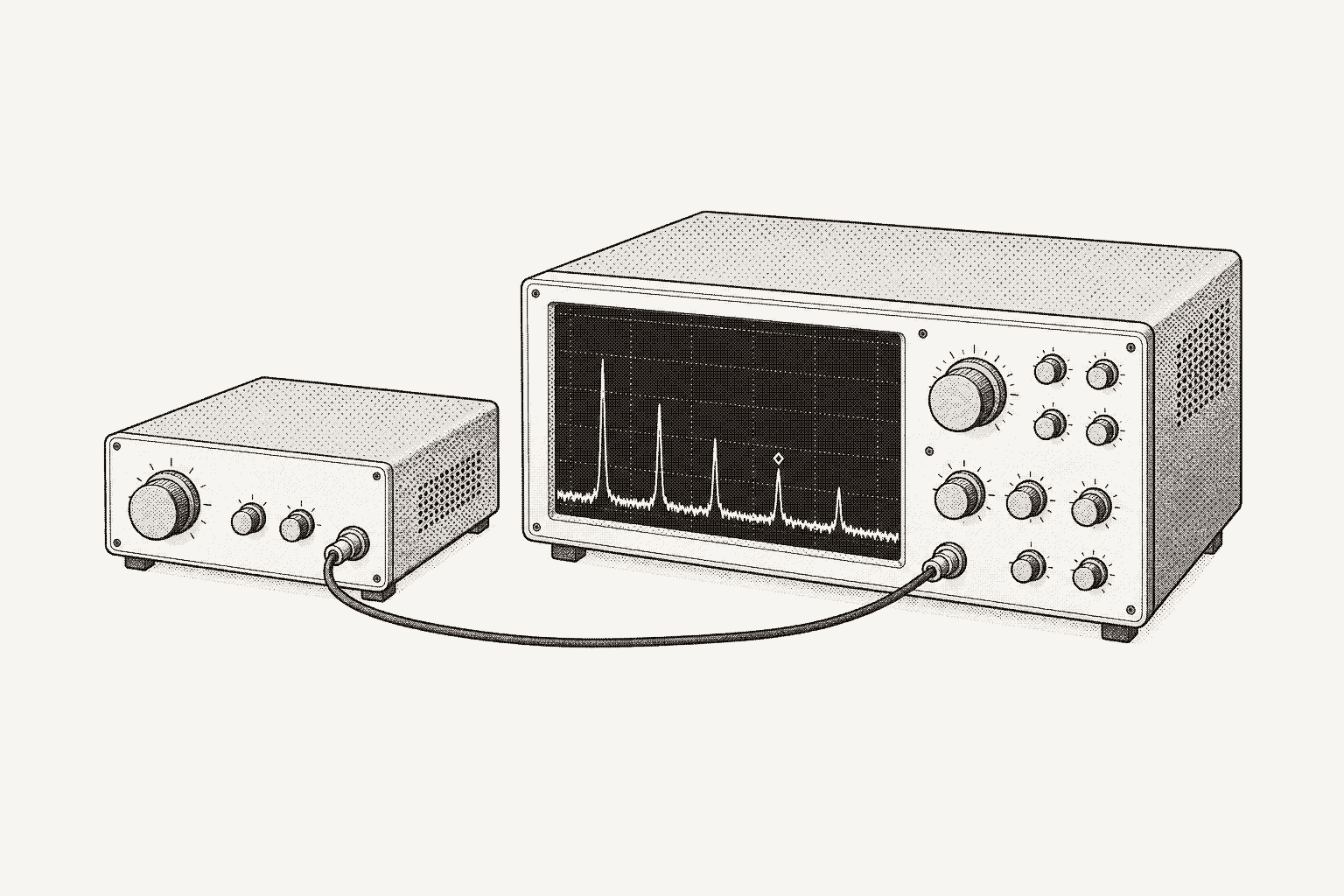
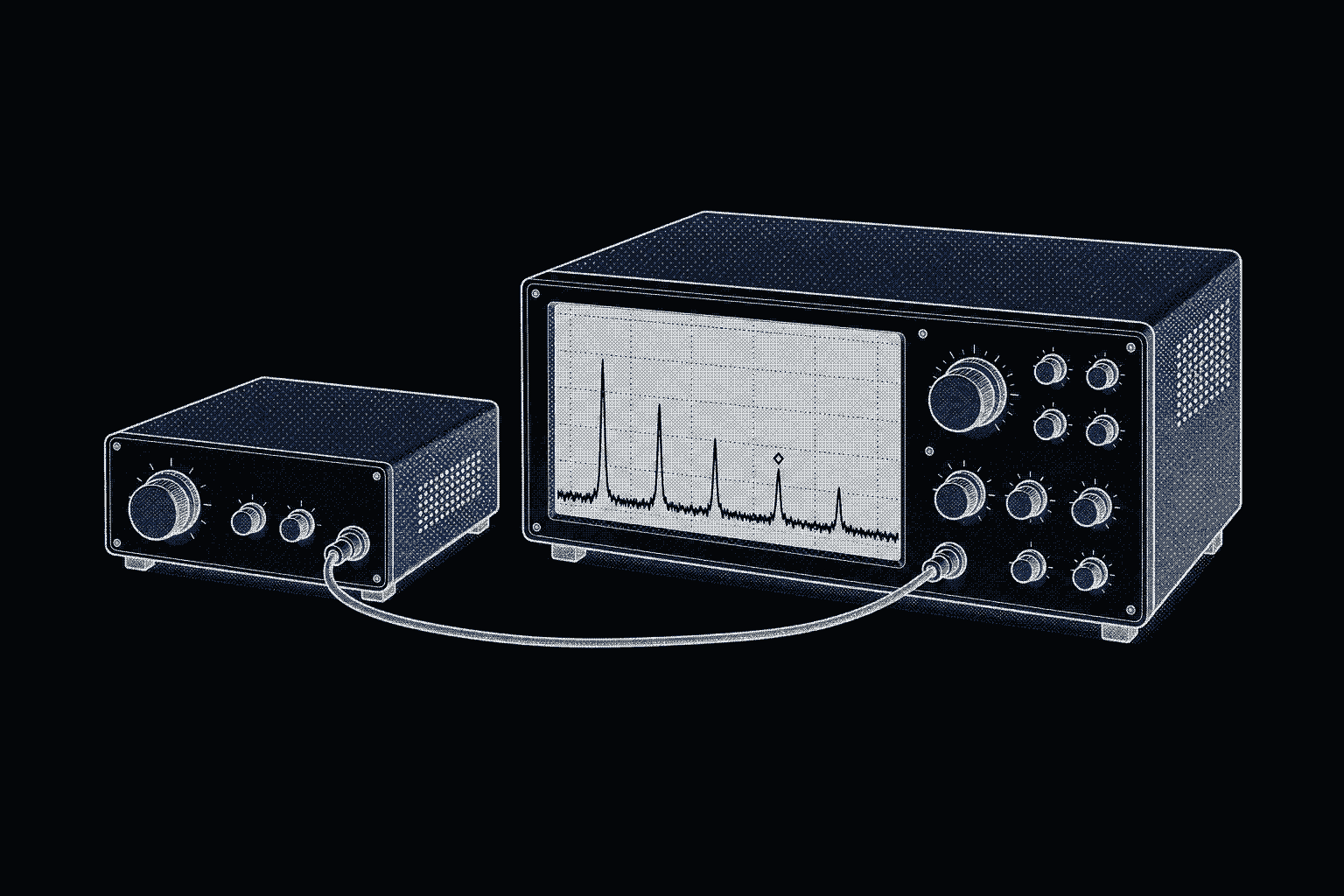
To simulate a spectrum analyzer for test automation, wire a simulated analyzer to a simulated source on a virtual bench and run the same SCPI your instrument script sends. Center, span, RBW, detectors, trace modes, markers and :TRACe:DATA? all answer, and every level can be checked against a closed form.
EdgeSim is the open-source bench simulator from Galois Labs: simulated instruments wired into simulated benches that PyVISA scripts, pytest, galois-edge and AI agents can't tell from real hardware. EdgeSim's open-source release, with the edgesim package and its example benches, is coming soon; every code block below was run on EdgeSim 0.2.0 with PyVISA 1.16.2 and Python 3.13 on October 7, 2026, against the specan.bench.yaml example bench. In that bench a function generator, sim-awg-1, puts a 100 kHz square wave on RF_IN, and a second, sim-awg-2, puts a 10 MHz-class sine on REF_IN. The sources are EdgeSim's analyzer profile, its behavior module and the semantics contract; nothing here was measured on a real analyzer, and the analyzer is one virtual instrument for the whole class. The EdgeSim announcement covers the other instrument classes, and RF signal generator simulation measures modulated carriers with this analyzer. Évariste, the agent in the Galois platform, does the same work in a later section.
What does the simulated analyzer compute?
The analyzer reads the net on RF_IN, not samples. A net carries a description, and the analyzer turns it into lines and noise and draws them through a Gaussian resolution filter over the trace points.
| What is on RF_IN | How the analyzer reads it |
|---|---|
| Sines, and nested terms of sines | Lines at each term's frequency, power V²/2R into 50 Ω |
| Square and ramp | Exact Fourier series: every harmonic is a line |
| Arb, PRBS and clipped signals | A windowed FFT, with a record length set by the RBW |
noise(σ) terms | White noise up to a stated band, so a density of σ²/B |
| The receiver itself | kT0·F·NBW: -174 dBm/Hz, plus the noise figure (24 dB), plus the attenuation, over 1.0645 × RBW |
noise() takes no bandwidth argument, so the band over which a noise term is white comes from a latent receiver setting, 7.5 GHz by default. The RBW filter is Gaussian with a -3 dB power width equal to the RBW, on a 1-3-10 ladder from 1 Hz to 3 MHz. Frequencies run from 0 to 7.5 GHz.
Two properties matter to test code. The trace is a pure function of the settings, the nets RF_IN carried since the last restart, the bench seed and the sweep counter, so two reads at one virtual instant are byte-identical. And the model is an ideal receiver: no level-accuracy ripple, no compression, no zero span, no tracking generator and no measurement applications. Tests here prove code, not an analyzer's accuracy.
The console, edgesim tui, draws that trace in its SPECTRUM box from the same model, with the marker as a diamond on the line, and while the sweep runs continuously it draws a new sweep, with new noise, every sweep time of virtual time. The trace is the :TRACe:DATA? reply, one dBm value per point from the start to the stop frequency.
Which bench puts a square wave on RF_IN?
The bench is a topology file plus ext.sim bags, the file the Galois cloud editor draws. The state of its three instruments is the part that matters:
# sim-awg-1: a 100 kHz square, 1 Vpp, output on -> analyzer RF_IN
state: {source.function: SQUare, source.frequency: 100000.0, source.amplitude: 1.0, output.enabled: true}
# sim-awg-2: 10 MHz + 20 Hz, 2 ppm high -> analyzer REF_IN
state: {source.frequency: 10000020.0, source.amplitude: 1.0, output.enabled: true}
# sim-specan-1: 0 to 1 MHz, reference level 10 dBm, locked to REF_IN
state: {frequency.center: 500000.0, frequency.span: 1000000.0, amplitude.ref_level: 10.0, timebase.source: EXTernal}
Validate it, then print what the solver made of the wiring:
edgesim validate specan.bench.yaml; echo "exit $?"exit 0import edgesim
with edgesim.open_bench("specan.bench.yaml") as world:
for net in world.nets():
print(net.id, net.members, "driver", net.driver)
for c in net.descriptor["components"]:
print(" ", c["kind"], [round(a, 9) if isinstance(a, float) else a for a in c["args"][:5]])
print(" ops", net.descriptor["ops"])net-0 ('inst-awg-sim1:OUT1', 'inst-specan-sim1:RF_IN') driver inst-awg-sim1:OUT1
dc [0.0]
square [100000.0, 0.25, 0.0, 0.5]
ops []
net-1 ('inst-awg-sim2:OUT1', 'inst-specan-sim1:REF_IN') driver inst-awg-sim2:OUT1
dc [0.0]
sine [10000020.0, 0.25, 0.0, 0.0]
ops []The square's arguments are frequency, amplitude, offset and duty. The generator's 1 Vpp is an open-circuit 0.5 V peak, and the 50 Ω input takes half, so the net carries 0.25 V. That number is the whole closed form: harmonic n of a square of amplitude A has peak 4A/(πn), and into 50 Ω its power is V²/2R.
The PyVISA path is the one the instrument script uses. A bench in the @edgesim resource manager opens one socket per instrument, and the two generators answer *IDN? alike, so find the analyzer by its model:
import pyvisa

rm = pyvisa.ResourceManager("specan.bench.yaml@edgesim")
for address in rm.list_resources():
    inst = rm.open_resource(address, read_termination="\n", write_termination="\n")
    print(address, inst.query("*IDN?"))
    if "SIM-SPECAN-1" in inst.query("*IDN?"):
        break
inst.write(":CALC:MARK:MAX")
print("peak:", inst.query(":CALC:MARK:X?"), "Hz,", inst.query(":CALC:MARK:Y?"), "dBm")
rm.close()TCPIP0::127.0.0.1::5025::SOCKET GALOIS,SIM-AWG-1,SIM00001,edgesim-1
TCPIP0::127.0.0.1::5026::SOCKET GALOIS,SIM-AWG-1,SIM00001,edgesim-1
TCPIP0::127.0.0.1::5027::SOCKET GALOIS,SIM-SPECAN-1,SIM00001,edgesim-1
peak: +1.00000000000000E+05 Hz, +5.700255E-02 dBmVirtual time matters for trace modes, and a PyVISA session cannot move it. The rest of this guide opens the bench in process and wraps the analyzer's SCPI in a small helper, so advance() can move the clock:
from contextlib import contextmanager

import numpy as np

import edgesim

SA, AWG, REF = "sim-specan-1", "sim-awg-1", "sim-awg-2"


class Rig:
    def __init__(self, world):
        self.world = world

    def ask(self, cmd: str, inst: str = SA) -> str:
        reply = self.world.scpi(inst, cmd)
        return "" if reply is None else reply.decode().strip()

    def num(self, cmd: str, inst: str = SA) -> float:
        return float(self.ask(cmd, inst))

    def errors(self) -> list[str]:
        out = []
        while not (e := self.ask("SYST:ERR?")).startswith("0,"):
            out.append(e)
        return out

    def trace(self) -> tuple[np.ndarray, np.ndarray]:
        """Frequency (Hz) and level (dBm) of every point, from the settings the analyzer reports."""
        start, stop = self.num(":SENS:FREQ:STAR?"), self.num(":SENS:FREQ:STOP?")
        y = np.array([float(v) for v in self.ask(":TRAC:DATA? TRACE1").split(",")])
        return np.linspace(start, stop, len(y)), y

    def advance(self, seconds: float) -> None:
        self.world.advance(seconds)


@contextmanager
def open_rig(bench: str):
    with edgesim.open_bench(bench) as world:
        yield Rig(world)
How do center, span, RBW, VBW and sweep time couple?
Span and center are primary; start and stop follow them. RBW, VBW, sweep time and attenuation each have an auto rule, and a manual value turns that coupling off.
| Setting | Auto rule | A manual value |
|---|---|---|
| RBW | span / 100, snapped to the 1-3-10 ladder | Snaps to the nearest step, auto off |
| VBW | Equal to the RBW | Snaps to the nearest step, auto off |
| Sweep time | 2.5 × span / (RBW × min(RBW, VBW)), at least 1 ms | Taken as given, auto off |
| Attenuation | Keeps the reference level at -10 dBm at the mixer, in 2 dB steps | Taken as given, auto off |
from rig import open_rig


def settings(r, label: str) -> None:
    print(f"{label}")
    print(f"  center {r.num(':SENS:FREQ:CENT?'):.0f} Hz, span {r.num(':SENS:FREQ:SPAN?'):.0f} Hz, "
          f"RBW {r.num(':SENS:BAND:RES?'):.0f} Hz (auto {r.ask(':SENS:BAND:RES:AUTO?')}), "
          f"VBW {r.num(':SENS:BAND:VID?'):.0f} Hz (auto {r.ask(':SENS:BAND:VID:AUTO?')})")
    print(f"  sweep {r.num(':SENS:SWE:TIME?'):.6g} s (auto {r.ask(':SENS:SWE:TIME:AUTO?')}, UNCal {r.ask(':SENS:SWE:TIME:UNC?')}), "
          f"reference level {r.num(':DISP:WIND:TRAC:Y:SCAL:RLEV?'):.0f} dBm, "
          f"attenuation {r.num(':SENS:POW:RF:ATT?'):.0f} dB (auto {r.ask(':SENS:POW:RF:ATT:AUTO?')}), "
          f"overload {r.ask(':SENS:POW:RF:OVER?')}")


with open_rig("specan.bench.yaml") as r:
    settings(r, "bench start")
    r.ask(":SENS:FREQ:CENT 200e3")                        # start would be negative: the window slides
    print(f"center 200 kHz asked, center now {r.num(':SENS:FREQ:CENT?'):.0f} Hz")
    r.ask(":SENS:FREQ:SPAN 10e6"); r.ask(":SENS:FREQ:CENT 5e6")
    settings(r, "span 10 MHz, then center 5 MHz")
    r.ask(":SENS:BAND:RES 2000")
    settings(r, "RBW 2 kHz asked")
    r.ask(":SENS:SWE:TIME 0.05")
    settings(r, "sweep time 50 ms asked")
    r.ask(":SENS:SWE:TIME:AUTO ON"); r.ask(":SENS:BAND:RES:AUTO ON")
    r.ask(":DISP:WIND:TRAC:Y:SCAL:RLEV -20")
    settings(r, "couplings back on, reference level -20 dBm")
    r.ask(":DISP:WIND:TRAC:Y:SCAL:RLEV 10")
    settings(r, "reference level 10 dBm again")
print(r.errors())bench start
center 500000 Hz, span 1000000 Hz, RBW 10000 Hz (auto 1), VBW 10000 Hz (auto 1)
sweep 0.025 s (auto 1, UNCal 0), reference level 10 dBm, attenuation 20 dB (auto 1), overload 0
center 200 kHz asked, center now 500000 Hz
span 10 MHz, then center 5 MHz
center 5000000 Hz, span 10000000 Hz, RBW 100000 Hz (auto 1), VBW 100000 Hz (auto 1)
sweep 0.0025 s (auto 1, UNCal 0), reference level 10 dBm, attenuation 20 dB (auto 1), overload 0
RBW 2 kHz asked
center 5000000 Hz, span 10000000 Hz, RBW 3000 Hz (auto 0), VBW 3000 Hz (auto 1)
sweep 2.77778 s (auto 1, UNCal 0), reference level 10 dBm, attenuation 20 dB (auto 1), overload 0
sweep time 50 ms asked
center 5000000 Hz, span 10000000 Hz, RBW 3000 Hz (auto 0), VBW 3000 Hz (auto 1)
sweep 0.05 s (auto 0, UNCal 1), reference level 10 dBm, attenuation 20 dB (auto 1), overload 0
couplings back on, reference level -20 dBm
center 5000000 Hz, span 10000000 Hz, RBW 100000 Hz (auto 1), VBW 100000 Hz (auto 1)
sweep 0.0025 s (auto 1, UNCal 0), reference level -20 dBm, attenuation 0 dB (auto 1), overload 1
reference level 10 dBm again
center 5000000 Hz, span 10000000 Hz, RBW 100000 Hz (auto 1), VBW 100000 Hz (auto 1)
sweep 0.0025 s (auto 1, UNCal 0), reference level 10 dBm, attenuation 20 dB (auto 1), overload 0
[]The arithmetic is the rule. A 1 MHz span gives a 10 kHz RBW and 2.5 × 10⁶ / (10⁴ × 10⁴) = 0.025 s. A 10 MHz span gives 100 kHz and 2.5 ms. A 2 kHz request snaps to 3 kHz, which leaves the VBW coupled at 3 kHz and stretches the sweep to 2.5 × 10⁷ / (3000 × 3000) = 2.778 s.
Center slides. Centering at 200 kHz on a 1 MHz span would put the start at -300 kHz, so the window slides and the center reads 500 kHz, with no error queued. Set the span first, then the center.
A short manual sweep time is flagged. At 50 ms against an auto 2.778 s, UNCal reads 1; the swept-filter widening itself is not modeled.
The reference level moves the attenuation, not the readings. At -20 dBm the auto attenuation falls to 0 dB and overload reads 1: the square's total power is 0.25² / 50 = 1.25 mW, +0.97 dBm, above the -10 dBm the first mixer takes. Readings stay uncompressed. Check the flag after any level change: it tells a script that the setup would overload a real front end.
How do I read :TRACe:DATA? and walk the markers?
:TRACe:DATA? TRACE1 returns comma-separated dBm, one value per point. Marker 1 reads the trace: :CALCulate:MARKer:MAXimum puts it on the highest peak, :CALCulate:MARKer:MAXimum:NEXT on the highest peak below the current one, and :CALCulate:MARKer:Y? reads its level. A peak must stand 6 dB above the valleys on both sides (the excursion) and exceed the threshold, which defaults to -130 dBm, below the floor. Raise it to keep floor noise out of the peak list.
import math

from rig import open_rig

A_V, R_OHM = 0.25, 50.0   # the square's amplitude on the net (nets.py), the analyzer's input impedance


def line_dbm(n: int) -> float:
    """Level of odd harmonic n of a square wave of amplitude A: peak 4A/(pi n), power V^2 / 2R, in dBm."""
    return 10 * math.log10((4 * A_V / (math.pi * n)) ** 2 / (2 * R_OHM) / 1e-3)


with open_rig("specan.bench.yaml") as r:
    f, y = r.trace()
    print(f"{len(y)} points, {f[0]:.0f} to {f[-1]:.0f} Hz, highest point {y.max():+.3f} dBm at {f[y.argmax()]:.0f} Hz")

    r.ask(":CALC:MARK:PEAK:THR -30")                     # keep the noise floor out of the peak list
    print(" n   marker Hz   counter Hz    marker dBm   closed form   difference")
    for n in (1, 3, 5, 7, 9):
        r.ask(":CALC:MARK:MAX" if n == 1 else ":CALC:MARK:MAX:NEXT")
        x, level, counted = r.num(":CALC:MARK:X?"), r.num(":CALC:MARK:Y?"), r.num(":CALC:MARK:FCO:X?")
        print(f"{n:2d}  {x:10.0f}  {counted:11.1f}  {level:+10.4f}  {line_dbm(n):+12.4f}  {level - line_dbm(n):+10.4f}")
    r.ask(":CALC:MARK:MAX:NEXT")                         # nothing is left above the threshold
print("after the ninth:", r.errors())1001 points, 0 to 1000000 Hz, highest point +0.057 dBm at 100000 Hz
n marker Hz counter Hz marker dBm closed form difference
1 100000 99999.8 +0.0570 +0.0570 +0.0000
3 300000 299999.4 -9.4854 -9.4854 +0.0000
5 500000 499999.0 -13.9224 -13.9224 -0.0000
7 700000 699998.6 -16.8450 -16.8450 -0.0000
9 900000 899998.2 -19.0279 -19.0278 -0.0000
after the ninth: ['-200,"Execution error"']The fundamental is +0.057 dBm, the third harmonic is 9.54 dB below it and the fifth 13.98 dB, which is 20·log10(n). The differences are zero to the digits shown because the analytic path computes the same Fourier series the check does. The check proves the code that finds the bin, applies the units and orders the peaks; a real analyzer adds level error.
The counter column shows the reference. :CALCulate:MARKer:FCOunt:X? reads the strongest line near the marker the way an ideal counter does. The analyzer is locked to the second generator's 10 MHz + 20 Hz, so it inherits its +2 ppm and shows every frequency divided by 1.000002: 100,000 Hz reads 99,999.8 Hz. The exact error is latent, so a script infers it from the counter.
Next-peak ends with -200. After the ninth harmonic nothing is left above -30 dBm, so the search queues -200 "Execution error" and leaves the marker where it was.
With the peak threshold at -30 dBm, each next-peak search hops the marker diamond to the next odd harmonic of the 100 kHz square, and the readout falls from 0.06 dBm at 100 kHz to -13.92 dBm at 500 kHz and -16.84 dBm at 700 kHz.
On the trace the diamond hops from peak to peak, and its readout carries each level the query returns.
How do the four detectors and three trace modes behave?
The detector reduces the samples in one trace point's bucket to one value: SAMPle takes one sample, POSitive the largest, AVERage the voltage average and RMS the power average. The trace mode accumulates sweeps: WRITe shows the newest, AVERage the mean of the newest :SENSe:AVERage:COUNt, MAXHold the largest since the restart. The detector shows on noise; a line reads alike on all four. floor.py puts 101 points across a quiet 100 kHz between the 100 kHz and 300 kHz lines, so each point covers ten 100 Hz resolution cells, and compares each detector with kT0·F·NBW:
import math

import numpy as np

from rig import open_rig

K_T0_DBM_HZ, NOISE_FIGURE_DB = -174.0, 24.0     # the model's rounded kT0 and the default noise figure
NBW_FACTOR = math.sqrt(math.pi / (4 * math.log(2)))   # noise bandwidth of the Gaussian RBW filter, 1.0645 RBW


def floor_dbm(rbw_hz: float, atten_db: float) -> float:
    return K_T0_DBM_HZ + NOISE_FIGURE_DB + atten_db + 10 * math.log10(NBW_FACTOR * rbw_hz)


def mean_power_dbm(y: np.ndarray) -> float:
    return float(10 * np.log10(np.mean(10 ** (y / 10))))


with open_rig("specan.bench.yaml") as r:
    r.ask(":SENS:FREQ:SPAN 100e3"); r.ask(":SENS:FREQ:CENT 200e3")
    r.ask(":SENS:SWE:POIN 101"); r.ask(":SENS:BAND:RES 100")
    print(f"RBW {r.num(':SENS:BAND:RES?'):.0f} Hz, attenuation {r.num(':SENS:POW:RF:ATT?'):.0f} dB, "
          f"kT0*F*NBW = {floor_dbm(100, 20):+.2f} dBm")
    print("detector   floor mean dBm   scatter dB   minus theory   300 kHz line dBm")
    for det in ("SAMPle", "POSitive", "AVERage", "RMS"):
        r.ask(f":SENS:DET:FUNC {det}")
        r.ask(":SENS:FREQ:CENT 200e3")
        _, y = r.trace()
        r.ask(":SENS:FREQ:CENT 300e3")                    # the third harmonic sits on the middle point
        _, line = r.trace()
        print(f"{det:9s}  {y.mean():+13.2f}   {y.std():10.2f}   {y.mean() - floor_dbm(100, 20):+12.2f}   {line.max():+14.4f}")
    r.ask(":SENS:FREQ:CENT 200e3")

    # The floor with the RMS detector, at four attenuator settings, at 1001 points.
    r.ask(":SENS:SWE:POIN 1001"); r.ask(":SENS:DET:FUNC RMS"); r.ask(":SENS:BAND:RES 1000")
    print("attenuation   floor dBm (mean power)   kT0*F*NBW")
    for att in (0, 10, 20, 30):
        r.ask(f":SENS:POW:RF:ATT {att}")
        _, y = r.trace()
print(f"{att:9d} dB {mean_power_dbm(y):+14.2f} {floor_dbm(1000, att):+22.2f}")RBW 100 Hz, attenuation 20 dB, kT0*F*NBW = -109.73 dBm
detector floor mean dBm scatter dB minus theory 300 kHz line dBm
SAMPle -112.07 5.58 -2.35 -9.4859
POSitive -103.85 1.36 +5.87 -9.4854
AVERage -110.85 0.77 -1.12 -9.4859
RMS -109.77 0.87 -0.05 -9.4859
attenuation floor dBm (mean power) kT0*F*NBW
0 dB -119.74 -119.73
10 dB -110.10 -109.73
20 dB -99.46 -99.73
30 dB -89.75 -89.73RMS reads the thermal floor. It averages power, and at -109.77 dBm it sits 0.05 dB from kT0·F·NBW. POSitive takes the largest of ten cells and reads 5.87 dB high, the number to expect when a script mixes a peak detector into a noise measurement. SAMPle and AVERage read low, 2.35 and 1.12 dB, because the display averages the log of noise power, which the model documents as 2.51 dB below the power.
A steady line does not care. The third harmonic reads -9.485 dBm on all four.
Attenuation raises the floor dB for dB. Each 10 dB step moves the mean floor 10 dB, within 0.4 dB of the arithmetic; a trace mean is an estimate over about a hundred independent cells.
The model has four detectors. :SENSe:DETector:FUNCtion QPEak is refused with -224 (see the error table below), so a script written for a quasi-peak scan finds out at the setup line, not in the data.
Trace modes need sweeps, and sweeps need virtual time. In continuous mode the trace is the sweep the virtual clock has reached since the last restart, and a mode change restarts it. modes.py advances the clock explicitly and compares the three modes on the floor, then moves the source from 100 kHz to 150 kHz partway through:
import numpy as np

from rig import AWG, open_rig


def level_at(f, y, hz):
    return float(y[int(np.argmin(np.abs(f - hz)))])


with open_rig("specan.bench.yaml") as r:
    r.ask(":SENS:DET:FUNC SAMP")
    # 1. The floor: a quiet 100 kHz stretch, sample detector, one trace per mode after ten sweeps.
    r.ask(":SENS:FREQ:SPAN 100e3"); r.ask(":SENS:FREQ:CENT 200e3"); r.ask(":SENS:BAND:RES 1000")
    r.ask(":SENS:AVER:COUN 10")
    sweep = r.num(":SENS:SWE:TIME?")
    print(f"sweep time {sweep} s; floor between the lines, ten sweeps per mode")
    _, first = r.trace()
    _, again = r.trace()
    print(f"  two reads at one virtual instant are identical: {np.array_equal(first, again)}")
    for mode in ("WRITe", "AVERage", "MAXHold"):
        r.ask(f":TRAC:TYPE {mode}")                  # a mode change restarts the trace
        r.advance(10.5 * sweep)
        _, y = r.trace()
        print(f"  {mode:8s} mean {y.mean():+7.2f} dBm   scatter {y.std():5.2f} dB")

    # 2. A source that moves: 100 kHz for twenty sweeps, then 150 kHz for twenty.
    r.ask(":SENS:FREQ:SPAN 1e6"); r.ask(":SENS:FREQ:CENT 5e5"); r.ask(":SENS:BAND:RES 10e3")
    r.ask(":SENS:DET:FUNC POS"); r.ask(":SENS:AVER:COUN 40")
    sweep = r.num(":SENS:SWE:TIME?")
    print(f"sweep time {sweep} s; level at 100 kHz and at 150 kHz after the source moves")
    for mode in ("WRITe", "AVERage", "MAXHold"):
        r.ask(f":SOUR1:FREQ 100000", AWG)
        r.ask(f":TRAC:TYPE {mode}")
        r.advance(20.5 * sweep)
        r.ask(f":SOUR1:FREQ 150000", AWG)
        r.advance(20 * sweep)
        f, y = r.trace()
        print(f"  {mode:8s} 100 kHz {level_at(f, y, 100e3):+8.2f} dBm   150 kHz {level_at(f, y, 150e3):+8.2f} dBm")
    r.ask(":TRAC:CLE")
    print("  after :TRACe:CLEar, held mode, no time passed:", end=" ")
    f, y = r.trace()
    print(f"100 kHz {level_at(f, y, 100e3):+8.2f}   150 kHz {level_at(f, y, 150e3):+8.2f}")
print(r.errors())sweep time 0.25 s; floor between the lines, ten sweeps per mode
two reads at one virtual instant are identical: True
WRITe mean -102.09 dBm scatter 5.49 dB
AVERage mean -102.34 dBm scatter 1.75 dB
MAXHold mean -95.37 dBm scatter 1.77 dB
sweep time 0.025 s; level at 100 kHz and at 150 kHz after the source moves
WRITe 100 kHz -100.08 dBm 150 kHz +0.06 dBm
AVERage 100 kHz -43.01 dBm 150 kHz -47.81 dBm
MAXHold 100 kHz +0.06 dBm 150 kHz +0.06 dBm
after :TRACe:CLEar, held mode, no time passed: 100 kHz -89.82 150 kHz +0.06
[]Averaging cuts the scatter by √N. Ten sweeps take the scatter from 5.49 to 1.75 dB, and 5.49 / √10 = 1.74. The mean stays put.
Max hold raises the floor. The largest of ten sweeps sits 6.7 dB above one sweep, with the scatter of an average. Use it for intermittent emitters, not for noise-floor figures.
The three modes remember differently. After the source moves, WRITe shows only the new line, MAXHold shows both at +0.06 dBm, and AVERage blends them: the newest 40 sweeps held about 20 at each frequency, so each line reads about halfway down from its level in dB. A :TRACe:CLEar forgets the old line.
Time is part of the setup. A trace that has not been given virtual time shows the first sweep. A script that expects an average or a hold must advance the clock, or take single sweeps with :INITiate:CONTinuous OFF and :INITiate, which takes the sweep time once per average.
How does the FFT path read PRBS, arb and clip?
Sines, squares and ramps are lines. A pseudo-random bit stream is not, so the analyzer materializes the signal and reads it through a windowed FFT, with a record long enough for the RBW. The AWG has no PRBS function, so a small profile adds one source, an order-7 sequence with a settable rate and level:
state:
  rate:  {type: float, unit: Hz, initial: 100000.0, min: 1000.0, max: 10000000.0}
  level: {type: float, unit: V, initial: 0.25, min: 0.0, max: 5.0}
ports:
  OUT: {dir: out, medium: voltage, z_ohm: 50.0}
sim:
  ports:
    OUT: "prbs(7, state.rate, state.level)"
The arguments of prbs are order, bit rate, amplitude and an optional offset. The profile was linted with galois-profiles lint profiles and the bench validated with edgesim validate prbs.bench.yaml --profile-dir profiles; both exited 0. A bench with that source on RF_IN and the analyzer on 0 to 200 kHz carries the net prbs [7, 100000.0, 0.125, ...], half the 0.25 V level across the 50 Ω input. An order-7 sequence repeats every 127 bits, so its spectrum is lines at k·R/127 under a sinc envelope, and line k has peak 2A·√128 / 127 · |sinc(k/127)|.
import math

import numpy as np

import edgesim
from rig import Rig

N, A_V, RATE_HZ = 127, 0.125, 100e3     # order 7, amplitude on the net, bit rate


def line_dbm(k: int) -> float:
    """Line k of an order-7 PRBS at k * rate / 127: peak 2A * sqrt(N + 1) / N * |sinc(k / N)|, into 50 ohm."""
    peak = 2 * A_V * math.sqrt(N + 1) / N * abs(np.sinc(k / N))
    return 10 * math.log10(peak**2 / 100 / 1e-3)


with edgesim.open_bench("prbs.bench.yaml", profile_dirs=["profiles"]) as world:
    r = Rig(world)
    r.ask(":SENS:FREQ:SPAN 20e3"); r.ask(":SENS:FREQ:CENT 10e3"); r.ask(":SENS:BAND:RES 100")
    f, y = r.trace()
    print(f"{len(y)} points, RBW {r.num(':SENS:BAND:RES?'):.0f} Hz, sweep time {r.num(':SENS:SWE:TIME?'):.0f} s")
    print("  k   line Hz   marker dBm   closed form   difference")
    for k in (1, 2, 5, 12, 20, 25):
        r.ask(f":CALC:MARK:X {k * RATE_HZ / N}")
        x, level = r.num(":CALC:MARK:X?"), r.num(":CALC:MARK:Y?")
print(f"{k:3d} {k * RATE_HZ / N:8.1f} {level:+9.3f} {line_dbm(k):+10.3f} {level - line_dbm(k):+10.3f}")1001 points, RBW 100 Hz, sweep time 5 s
k line Hz marker dBm closed form difference
1 787.4 -23.060 -23.046 -0.014
2 1574.8 -23.034 -23.049 +0.015
5 3937.0 -23.083 -23.067 -0.016
12 9448.8 -23.188 -23.173 -0.015
20 15748.0 -23.412 -23.402 -0.009
25 19685.0 -23.643 -23.606 -0.037The FFT path agrees with the closed form to 0.04 dB. The marker sits on the nearest 20 Hz bin, which accounts for most of the difference. The model's note adds one limit: an FFT estimate has no image rejection, so a line within three RBW of 0 Hz reads high.
When does the analyzer raise -221?
When the analyzer cannot draw a trace completely it draws what it can and queues -221 "Settings conflict" on every :TRACe:DATA? read until the settings change, never -241, which hosts read as a disconnect.
from rig import AWG, Rig, open_rig

import edgesim

# A 100 kHz square has about 100,000 lines in a 20 MHz window once it drops to 100 Hz: more than a trace holds.
with open_rig("specan.bench.yaml") as r:
    r.ask(":SOUR1:FREQ 100", AWG)
    r.ask(":SENS:FREQ:SPAN 20e6"); r.ask(":SENS:FREQ:CENT 10e6")
    _, y = r.trace()
    print(f"100 Hz square, 20 MHz span: {len(y)} points, highest {y.max():+.2f} dBm")
    print("  queue:", r.errors())
    _, y = r.trace()
    print("  read again, queue:", r.errors())

# A fast PRBS read at a 1 Hz RBW needs an FFT record longer than 2^20 samples: the trace is noise floor only.
with edgesim.open_bench("prbs.bench.yaml", profile_dirs=["profiles"]) as world:
    r = Rig(world)
    world.scpi("prbs-1", ":RATE 10e6")
    r.ask(":SENS:FREQ:SPAN 10e3"); r.ask(":SENS:FREQ:CENT 5e3"); r.ask(":SENS:BAND:RES 1")
    _, y = r.trace()
    print(f"10 Mb/s PRBS, RBW 1 Hz: highest {y.max():+.2f} dBm")
    print("  queue:", r.errors())
    r.ask(":SENS:BAND:RES 1000"); r.ask(":SENS:FREQ:SPAN 1e6"); r.ask(":SENS:FREQ:CENT 5e5")
    _, y = r.trace()
print(f"10 Mb/s PRBS, RBW 1 kHz: highest {y.max():+.2f} dBm, queue {r.errors()}")100 Hz square, 20 MHz span: 1001 points, highest +0.97 dBm
queue: ['-221,"Settings conflict; too many lines for one trace: the weakest were dropped"']
read again, queue: ['-221,"Settings conflict; too many lines for one trace: the weakest were dropped"']
10 Mb/s PRBS, RBW 1 Hz: highest -130.07 dBm
queue: ['-221,"Settings conflict; signal needs a longer FFT record than 2^20 samples at this RBW"']
10 Mb/s PRBS, RBW 1 kHz: highest -23.04 dBm, queue []The same PRBS at a 1 kHz RBW draws its lines at -23.04 dBm and the queue stays empty. A script that checks the queue after every :TRACe:DATA? catches both caps.
| Condition | What the trace holds | Message after "Settings conflict;" |
|---|---|---|
| More than 65,536 lines in the window, or over 2×10⁷ line-and-bin pairs | The strongest lines | too many lines for one trace: the weakest were dropped |
| An arb, PRBS or clipped signal needing an FFT record over 2²⁰ samples at the RBW | The noise floor only | signal needs a longer FFT record than 2^20 samples at this RBW |
EXTernal timebase, no 10 MHz sine within 10 ppm on REF_IN | Internal reference stays in use, lock flag 0 | external reference unusable: REF_IN needs a 10 MHz sine within 10 ppm, the analyzer stays on its internal reference |
| A max-hold older than its sweep limit | The newest sweeps (999 at 1001 points) | Queued once per restart |
Other refusals use their own codes:
from rig import AWG, REF, open_rig

with open_rig("specan.bench.yaml") as r:
    for label, cmd in [("span 1 Hz", ":SENS:FREQ:SPAN 1"), ("center 8 GHz", ":SENS:FREQ:CENT 8e9"),
                       ("RBW 0.5 Hz", ":SENS:BAND:RES 0.5"), ("detector QPEak", ":SENS:DET:FUNC QPEak")]:
        r.ask(cmd)
        print(f"{label:15s} -> {r.errors()}")
    r.ask(":CALC:MARK:PEAK:THR -30")
    r.ask(":OUTP1:STAT OFF", AWG)                          # the source off: no peak above -30 dBm
    r.ask(":CALC:MARK:MAX")
    print(f"{'peak, no signal':15s} -> {r.errors()}")
    r.ask(":OUTP1:STAT OFF", REF)                          # the reference off, then ask for it
    r.ask(":SENS:ROSC:SOUR INT"); r.ask(":SENS:ROSC:SOUR EXT")
print(f"{'EXT, no ref':15s} -> locked {r.ask(':SENS:ROSC:LOCK?')}, in use {r.ask(':SENS:ROSC:ACT?')}, {r.errors()[:1]}")span 1 Hz -> ['-222,"Data out of range"']
center 8 GHz -> ['-222,"Data out of range"']
RBW 0.5 Hz -> ['-222,"Data out of range"']
detector QPEak -> ['-224,"Illegal parameter value"']
peak, no signal -> ['-200,"Execution error"']
EXT, no ref -> locked 0, in use INT, ['-221,"Settings conflict; external reference unusable: REF_IN needs a 10 MHz sine within 10 ppm, the analyzer stays on its internal reference"']Range violations are -222, a value outside an allowed set is -224, and a failed peak search is -200. SCPI instrument automation with Python covers reading the error queue.
How do I run this in Galois with Évariste?
Galois is agent-driven test engineering for hardware teams: agents generate tests and instrument drivers, run them on real benches through the open-source galois-edge daemon, and turn the results into reports and a shared engineering record. The instrument library holds 573 profiles across 135 manufacturers, and EdgeSim plugs into galois-edge as an instrument backend, so Évariste works the virtual bench with the tools it uses on a real one. This section is a worked example, not a captured session.
Start the daemon with SIM_MODE on, SIM_BENCH at specan.bench.yaml and SIM_MARK_INSTRUMENTS=true, so list_instruments marks each instrument is_simulated. Open Évariste from the app sidebar (Ctrl+Shift+E) and ask "List connected instruments": the two generators and the analyzer appear. State the check with its limits:
On the virtual bench, set the spectrum analyzer to a 1 MHz span centered on 500 kHz and read the harmonics of the square wave on RF_IN. First write down the expected level of the first five odd harmonics from the Fourier series: the square is 0.25 V peak across 50 Ω. Then raise the peak threshold to -30 dBm, run a peak search and four next-peak searches, and read each marker's frequency and level. Stop and report if any level differs from your expected value by more than 0.05 dB or the analyzer queues an error. Check the overload flag after setting the reference level.
Draft. Évariste reads the analyzer's profile and drafts named commands. The first record:
name: "Square-wave harmonics on the virtual analyzer"
steps:
  - name: "Span 1 MHz"
    type: action
    config:
      instrument_id: "sim-specan-1"
      command_name: "frequency.span"
      parameters: { span: "1000000" }

  - name: "Center 500 kHz"
    type: action
    config:
      instrument_id: "sim-specan-1"
      command_name: "frequency.center"
      parameters: { frequency: "500000" }

  - name: "Peak threshold -30 dBm"
    type: action
    config:
      instrument_id: "sim-specan-1"
      command_name: "marker.peak.threshold"
      parameters: { threshold: "-30" }

  - name: "Peak search"
    type: action
    config:
      instrument_id: "sim-specan-1"
      command_name: "marker.peak.search"

  - name: "Marker level 1"
    type: measure
    config:
      instrument_id: "sim-specan-1"
      command_name: "marker.y"
      unit: "dBm"

  # next-peak search and marker level repeated four times; the comparison with the expected levels is Évariste's analysis
Review and approve. A draft cannot run until you approve it, and every edit is a new version with a diff. Check the span and center, the threshold against the floor, the number of next-peak steps and the tolerance (how to review an AI-generated test plan has the checklist).
Run and check. galois-edge runs the approved sequence against the virtual bench, and each step records its command, raw response and timestamps. The code path predicts the answer: +0.057, -9.485, -13.922, -16.845 and -19.028 dBm at 100, 300, 500, 700 and 900 kHz, all within tolerance. Check Évariste's figures against harmonics.py, and ask it to report the overload flag and the error queue with them.
One change. Ask for the same walk with a 0 dBm reference level and the attenuation on auto: the draft changes as a new version with a diff, and the run reports overload at 1.
The real analyzer. Bind the real analyzer in place of the virtual one, as a new version with its own diff and approval. The sequence keeps its steps; the expected levels come from the real source's measured amplitude, and the tolerance widens to the instrument's level accuracy. Then ask for "Generate a test report from the last run".
The sequence rehearsal gate is in build: every sequence will dry-run on a virtual bench built from the project's topology before approval, so a draft arrives with its marker arithmetic already exercised, and hosted virtual edge will run that bench without you starting a daemon.
You no longer write the PyVISA sessions, the marker loop, the comparison or the report script. The span, the threshold, the tolerance, the expected levels, review and approval, and the bench, from cabling the source to choosing the attenuation, stay yours.
| Step | Code path (this guide) | Galois with Évariste |
|---|---|---|
| Bench | specan.bench.yaml | The same file through SIM_MODE and SIM_BENCH |
| Known answer | line_dbm() | Expected levels first; markers compared within 0.05 dB |
| Setup | rig.py, coupling.py | Drafted named commands; settings in the objective |
| Walk | harmonics.py | Peak search, next-peak steps, marker levels |
| Review | Code review | Engineer approves the draft |
| Errors | r.errors() | Error queue reported with the results |
| Report | print() | "Generate a test report from the last run" |
What does a simulated analyzer never tell me, and when is plain code enough?
The model is an ideal receiver. Whatever it leaves out, the instrument and the bench decide:
| The simulation settles | The real analyzer and bench settle |
|---|---|
| Marker order, bin lookup, units and tolerance arithmetic | Level accuracy and frequency-response ripple |
That the script checks overload and the error queue | Compression and what an overload does to the readings |
| RBW, VBW and sweep-time coupling in the script's own math | The swept-filter widening behind UNCal |
| Detector choice against a known floor | Quasi-peak weighting for a compliance scan |
| Trace-mode logic, with virtual time under your control | Real sweeps, triggers and instrument timing |
Plain code is enough for one engineer, one analyzer and a marker routine already trusted on the bench: keep harmonics.py as a check that needs no instrument and run it in CI (hardware tests in CI). The simulation pays when the routine feeds a decision, when the analyzer is booked by someone else, and when several people run the same scan. A pass here proves the routine's logic against a model; only the real analyzer answers for the hardware.
Next, RF signal generator simulation puts a modulated carrier on this analyzer's input.
Frequently asked questions
- How do I simulate a spectrum analyzer for test automation?
- Wire a simulated analyzer to a simulated source in a bench file, then drive it with the SCPI your instrument script already sends: center, span, RBW, detector, trace mode, markers and :TRACe:DATA?. EdgeSim's analyzer reads the net on RF_IN as spectral lines plus noise, so a 100 kHz square wave reads its odd harmonics at levels you can check against 4A/(πn).
- Which detectors does the simulated spectrum analyzer have?
- SAMPle, POSitive, AVERage and RMS. On a noise floor at 100 Hz RBW they read 2.35 dB below, 5.87 dB above, 1.12 dB below and 0.05 dB below kT0·F·NBW in the run in this guide, and all four read a steady line alike. The model has no CISPR quasi-peak detector, and asking for QPEak is refused with error -224.
- How does a simulated analyzer compute the noise floor?
- The mean noise power in one resolution bandwidth is kT0·F·NBW: -174 dBm/Hz plus the noise figure (24 dB by default) plus the input attenuation, over a noise bandwidth of 1.0645 times the RBW. At 20 dB attenuation and a 100 Hz RBW that is -109.73 dBm, and the RMS detector read -109.77 dBm.
- When does the simulated spectrum analyzer return error -221?
- When it cannot draw a trace completely or a setting conflicts: more than 65,536 lines in the window, an arb, PRBS or clipped signal that needs an FFT record over 2^20 samples at the RBW, or EXTernal timebase without a usable 10 MHz reference. The trace is still returned, drawn as far as it can be, and the error repeats on every :TRACe:DATA? read until the settings change.
- Can Évariste test marker and RBW code on a virtual bench?
- Yes. Évariste, the agent in the Galois platform, drafts the sequence from a plain-English objective, writes the expected harmonic levels first and compares them with the markers the virtual bench returns. You approve the draft before it runs, and every edit is a new version with a diff. The same sequence then runs on the real analyzer through galois-edge. The automatic rehearsal gate before approval is in build.
Bring Galois to your bench.
The daemon is Apache-2.0, free forever. Enterprise runs in your cloud or on-prem.